Thoughts on geodata
I’ve not been coding a lot during the past month since I quit my job at Grafana Labs to take a stab at an extended vacation and thinking a bit about my next steps in life. I have however been spending some time at the computer working on a problem that have been a special interest of mine for quite a while: Mapping.
Maps have always fascinated me. A well-made map is like artwork that translates into a real life adventure. The terrain map made by Lantmäteriet (the Swedish Land Survey) is one of my favorite examples of that. It’s a map made for the scale 1:50 000 (half a meter on the map represents 25km in real life) with height curves and details about trails and landmarks suitable for wandering.
The general staff map (generalstabskartan) was originally made in the 1820s to provide a detailed and accurate map over all of Sweden, similar to the French Cassini maps produced during the 17th and 18th century. In the 1970s, the general staff map had become antiquated and was replaced by what would eventually come to be known as the terrain map.
My interest in this map could very well have ended around here, but thankfully some recent (2016, with additional data being made available by February 2025, see press release on open data funding from the land survey) development opening up land survey data. These days, the terrain map is all but replaced by raw map data being made available under the name of Topo50.
This enables anyone with QGIS and a little bit of time to create their own maps of Sweden using geodata. I quickly threw some Stockholm data at QGIS and made a quick draft for how I want to eventually render my map.
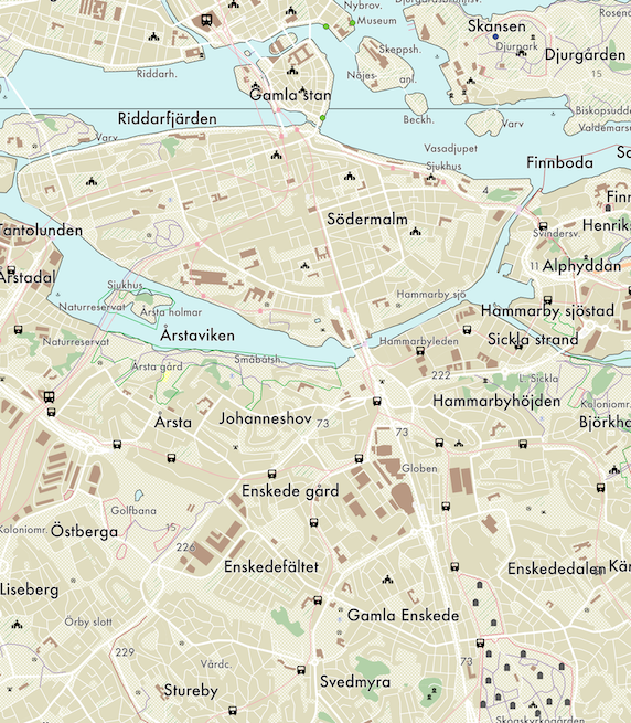
However, my goal isn’t to use QGIS. My goal is to take the long way around and try to understand the map on a different level than I believe I ever could without building my own map renderer. I’m working on a map renderer that is capable of rendering Topo50 map data into tilesets for Leaflet based on style sheets and configuration files.
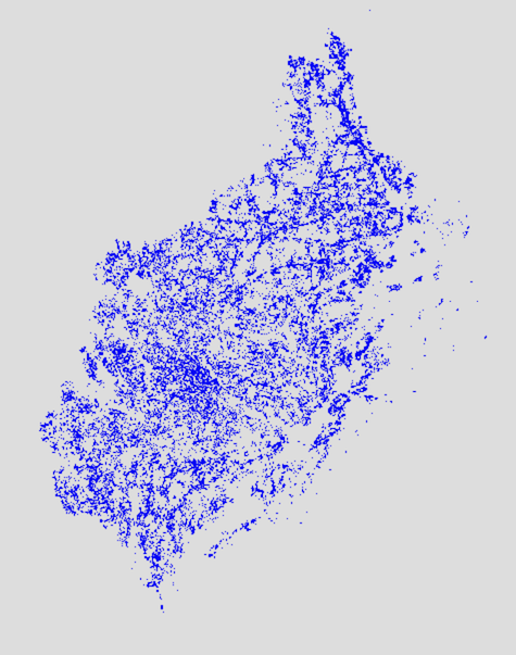
So far? It’s not much to look at, but this is what I have:
Getting here warranted utilizing some mathematics which I don’t understand. If you are into linear algebra, the mathematics and story behind it is quite well presented in LMV-rapport 2010:1 (sv)) and the main formulas are presented in “Gauss Conformal Projection (Transverse Mercator) — Krüger’s Formulas” (en).
The coordinates provided in the raw data are given in a meter based format based on SWEREF 99 TM. SWEREF 99 TM is a projection of coordinates that is intended to bring a high level of accuracy to mapping Sweden and match up to international standards. Thankfully, this means that the GRS80 reference ellipsoid (the shape of the virtual globe, since representing the shape of earth is hard and representing a random more or less squeezed ball is easier) originally used by WGS84 (the GPS coordinate system) is used for SWEREF 99 TM. SWEREF 99 is static to Sweden’s position on earth in 1989, so there is a small drift from WGS84, but not enough to cause anything near a problem on the scale of “hobbyist trying to render maps for hiking”-level.
The proximity to WGS84 coordinates means that I can ignore the differences in my calculations and place items as though their coordinates were provided in WGS84 originally. Phew.
The formulas I found for converting coordinates to their respective map tile at a certain zoom level requires having the longitude in degrees and the latitude in radians. Thankfully, Krüger’s formulas help with the conversion from coordinates on a plane onto an ellisoid.
The formulas are packed with magical numbers that I wouldn’t be able to make sense of, but the first example for the conversion I found at Trafiklab: Converting SWEREF99 to WGS84 had a text saying
Since this conversion is quite complicated, we recommend you use a library to do the heavy lifting.
…and I’m sure that’s sound advice, but I want to do it myself. I suspect the sample code wasn’t meant to be used as a reference, as it has a number of oddities (beyond mathematical rather than programmatic naming of variables, which can be ok for translating mathematical formulas to code):
- The dialect of the code is not clearly defined. When
sin(phi_star)^2is introduced toward the end of the snippet, the other exponents have been written using multiplicationn*n*n*nrather thann^4. Without knowing the programming language,sin(phi_star)^2can be either $\sin(\phi^\star) \oplus 2$ or $\sin(\phi^\star)^2$ as^is a popular token for bitwise xor. - The code lacks any kind of guiding whitespace or commentary that’d tell the user which operations are being performed and what their functions are. Latitude calculations and longitude calculations are intermixed almost at random.
deg_to_rad = 017453292519943295D. Pi is probably the most recognizable constant in the world, and this code would be so much more legible if it’d saydeg_to_rad = pi/180When reversing this operation at the end, pi makes an appearance, though in expanded form. I’d argue that’s better, as180 / 3.141592653589793is significantly more legible compared to57.29577951308232. Though why not introducepiat this point? I also have no idea what language would allow you to specify0.017453292519943295like that. Did they edit away the leading.?- There is repetition of the same operation without any hint or indication that such is the case. Let me expand that:
For example, there are eight occurrences of
$$ \alpha = \alpha_1c + \alpha_2c^2 + \alpha_3c^3 + \alpha_4c^4 $$
Namely:
$$ \begin{matrix} \alpha & c & \alpha_1 & \alpha_2 & \alpha_3 & \alpha_4\\ \hline \delta _1 & n & 1/2 & -2/3 & 37/96 & -1/360\\ \delta _2 & n & 0 & 1/48 & 1/15 & -437/1440\\ \delta _3 & n & 0 & 0 & 17/480 & -37/840\\ \delta _4 & n & 0 & 0 & 0 & 4397/161280\\ a^\star & e_2 & 1 & 1 & 1 & 1\\ b^\star * -6 & e_2 & 0 & 7 & 17 & 30\\ c^\star * 120 & e_2 & 0 & 0 & 224 & 889\\ d^\star * -1260 & e_2 & 0 & 0 & 0 & 4279\\ \end{matrix} $$
where
$$ f = \frac{1}{298.257222101}\\ n = \frac{f}{2 - f}\\ e_2 = f \times (2 - f)\\ $$
$f$ is a flattening factor provided for the ellipsoid. This is necessary as earth’s circumference is a bit bigger along the equator than the meridians.
Rather than
e2 = this.flattening * (2 - this.flattening)
n = this.flattening / (2 - this.flattening)
delta1 = n / 2 - 2 * n * n / 3 + 37 * n * n * n / 96 - n * n * n * n / 360
delta2 = n * n / 48 + n * n * n / 15 - 437 * n * n * n * n / 1440
delta3 = 17 * n * n * n / 480 - 37 * n * n * n * n / 840
delta4 = 4397 * n * n * n * n / 161280
Astar = e2 + e2 * e2 + e2 * e2 * e2 + e2 * e2 * e2 * e2
Bstar = -(7 * e2 * e2 + 17 * e2 * e2 * e2 + 30 * e2 * e2 * e2 * e2) / 6
Cstar = (224 * e2 * e2 * e2 + 889 * e2 * e2 * e2 * e2) / 120
Dstar = -(4279 * e2 * e2 * e2 * e2) / 1260
this could be expressed as
e2 := flattening * (2 - flattening)
n := flattening / (2 - flattening)
fn := func (n, a, b, c, d float64) float64 {
	return a*n + b*n*n + c*n*n*n + d*n*n*n*n
}

delta1 := fn(n, 1./2, -2./3, 37./96, -1./360)
delta2 := fn(n, 0, 1./48, 1./15, -437./1440)
delta3 := fn(n, 0, 0, 17./480, -37./840)
delta4 := fn(n, 0, 0, 0, 4397./161_280)
aStar := fn(e2, 1, 1, 1, 1)
bStar := fn(e2, 0, 7, 17, 30) / -6
cStar := fn(e2, 0, 0, 224, 889) / 120
dStar := fn(e2, 0, 0, 0, 4279) / -1260
Though unnecessary for our calculations, we could further generalize the function fn here to support any number of terms.
In my opinion it’s easier for the reader to detect that there is a pattern between the operations when applying some structure to the code. I noticed some open source projects implementing this algorithm align the terms with whitespacing. I’ve chosen to introduce new helper functions instead, this is a matter of taste and there’s no right or wrong. Legibility is highly subjective, but I think there are some general truths that can be considered.
When combining resources available by Trafiklab, Trafikverket, and studying pre-existing open source implementations in other languages I was able to write the functions I needed to convert values from SWEREF 99 TM coordinates to a geodesic format based on the GRS80 ellipsoid after having dissected the code snippets and math formulas a bit further.
You can find my implementation on GitHub, see dememorized/cassini.
Now that I have geodesic coordinates that mostly align with WGS84 from the raw geodata provided in SWEREF 99 TM, I want to… go back to a grid based system. This time, I’m interested in figuring out the boundaries between tiles for Leaflet, which use the format described by OpenStreetMaps’s wiki on Slippy map tilenames.
The tilenames contain three components, a x value for longitude, a y value for latitude, and a zoom-level z. The zoom-level z is a number for how many tiles the world should be divided into: z=0 has a single tile for the entire world, z=1 divides it into its north-west, north-east, south-west, and south-east corners, z=2 divides each corner again into 16 parts and so on. The number of tiles $f(z)$ at a certain zoom-level can be calculated using the following formula:
$$f(z)=2^{2z}$$
Open Street Maps’s wiki on Zoom levels have a good guide to how zoom levels work and which zoom levels are appropriate to use when representing various geographic features. For my project, zoom levels 13 and 14 are going to be the most relevant, but I’ll have to think about other zoom levels as well since users expect to be able to zoom into and out of a map. Lantmäteriet have four different topographical map data collections (1:50 000 being the finest and 1:1 000 000 the coarsest) which can be used to render out different zoom levels with appropriate amounts of details.
Note There’s a little bit of a cutoff here because I wrote this post in August and then sort of grew bored with this particular project. I thought some of you might be interested to see what I’ve built despite my own loss of motivation for it, which is why I choose to share this as-is.
References
- The Red Atlas: How the Soviet Union Secretly Mapped the World by John Davies and Alexander J Kent (9780226389578)
- “Gauss Conformal Projection (Transverse Mercator) — Krüger’s Formulas” (en)
- LMV-rapport 2010:1 (sv))